VI. Evaluate Algorithms
Overview
The evaluation process of Machine Learning algorithms is maybe the most important part of all. It is about evaluating the performance of the different neural nets trained for each HP/RDC combination. Not only does the evaluation tell you how good the predictions of the algorithms are, but you also get information on how robust and stable the algorithm will operate in the field.
Good to know
The performance of an algorithm (and the respective neural nets) should always be considered in the tension between two quantities:
- Variance of the input data (the more variance the better)
- Performance of the neural net (the higher the better)
The overview table compares the performance of the individual neural nets and gives you the possibility to export the neural net configuration for the BSEC library.
For Classification three performance indicators are shown for each neural net: Accuracy, F1 Score and False/Positive. For Regression you can choose between MSE, MSE%, RMSE,RMSE%, MAEand MAE%. Detailed information on these performance indicators can be found below.
Please note
As you progress through various testing configurations with the algorithm, it's important to be aware that deviations from the performance metrics observed during the training phase are quite normal. Algorithms, when exposed to diverse or unforeseen testing conditions, might exhibit variations in performance. This discrepancy is a common aspect of machine learning models and should be expected. Continuous training across a range of scenarios to better optimize your model's robustness and adaptability in real-world applications is recommended.
Performance Indicator (Classification)
Accuracy
The accuracy is the standard performance measurement for a classification algorithm. It tells you how likely it is that the algorithm will predict the correct class.
In other words it gives the ratio between correct and incorrect predictions. It is calculated by dividing the sum of the diagonal elements of the Confusion Matrix by the total sum of all elements (which is the amount of Validation Data used).
Macro-averaged F1 Score
The F1 Score is another performance indicator on how well the prediction of validation data samples is working. It comes in handy when class distributions are unevenly distributed and therefore accuracy values are harder to interpret.
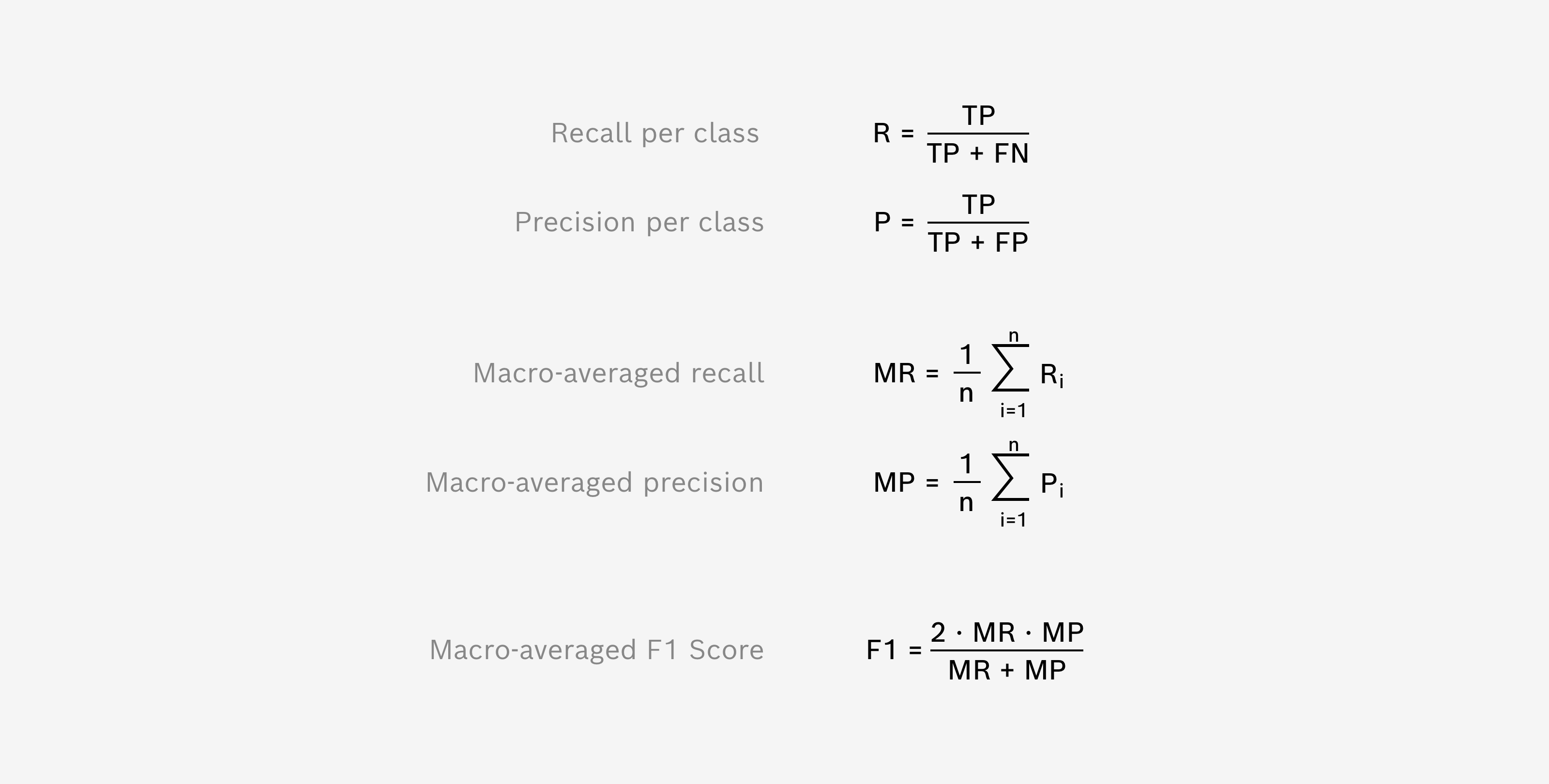
It is based on the recall and precision, two quantities that relate the True/Positive case with its false alarms. Recall relates between all correctly predicted elements to a given class and all elements that actually belong to this class. While Precision relates between all correctly predicted elements to a given class and all elements that were predicted to this class. Both values are calculated for each class and then averaged (so “called macro-averaging”). The shown F1 Score represents the harmonic mean of macro-averaged recall and precision.
Further information on performance measures
We follow the findings of Sokolova, Marina, and Guy Lapalme. "A systematic analysis of performance measures for classification tasks." Information processing & management 45.4 (2009): 427-437 in order to use F1 Score as a harmonic mean of macro-averaged recall and precision rather than calculating the macro-average of class independent F1 Scores.
Macro-averaged False/Positive rate
The False/Positive rate (also called miss rate) gives you an indication of how many false alarms (or more general: how many false predictions) will happen in your algorithm. Therefore a lower False/Positive rate indicates a better performance of the algorithm.
The False/Positive rate is defined as the relation between elements that belong to a different class, but have been falsely predicted to the given class (often called false alarms) and all elements predicted to the given class. The shown False/Positive rate is calculated as the macro-average of the class-specific False/Positive rates.
Performance Indicator (Regression)
Mean Square Error (MSE) and MSE in percent (MSE%)
MSE is a common performance metric for regression algorithms. It tells you how close the model's predictions are to the actual values, with lower values indicating better performance.
In essence, it calculates the average squared difference between predicted and actual values, meaning it heavily penalizes larger errors. This is computed by taking each error (difference between prediction and actual), squaring it (to remove any negative values), adding these squares together, and then taking the average of this sum across all n data points in the validation set.
MSE = (1/n) · Σ (y_actual - y_pred)^2
MSE% is very similar to MSE, but normalized in relation to the maximum used value in training for the respective target (Meta Data key) and expressed as a percentage.
MSE% = (MSE / value_max)
Root Mean Square Error (RMSE) and RMSE in percent (RMSE%)
RMSE is the standard option and a widely-used metric for evaluating the performance of regression models, since it is in the same units as the target variable, making it easier to interpret and understand. Root Mean Spuared Error (RSME) is very similar to MSE, but taken the square root of it.
RMSE = √ MSE
RMSE% is very similar to RMSE, but normalized in relation to the maximum used value in training for the respective target (Meta Data key) and expressed as a percentage.
RMSE% = (RMSE / value_max)
Mean Absolut Error (MAE) and MAE in percent (MAE%)
MAE calculates the average of the absolute differences between the predicted and actual values. It tells you how far off your predictions are from the actual values on average, with smaller values indicating better accuracy.
Unlike the MSE, it doesn't square the errors, so it doesn't give extra weight to larger errors and may therefore be more robust to outliers.
MAE = (1/n) · Σ |y_actual – y_pred|
MAE% is very similar to RMSE, but normalized in relation to the maximum used value in training for the respective target (Meta Data key) and expressed as a percentage.
MAE% = (MAE / value_max)
BSEC Export
Before you export a configuration file, please check that you have successfully trained and Algorithm.
Recap: How to train an algorithm?
- Go to the “Specimen Collection” section and configure your Development Kit Board for recording data using the “Configure BME Board” feature
- Record data using the Development Kit Board with the configuration files exported from BME AI-Studio Desktop
- Import the recorded data into BME AI-Studio Desktop
- Got to the “My Algorithms” sections and Create a new (classification) algorithm
- Create at least two classes and assign the previously recorded data in the form of specimens to the respective classes
- Train the algorithm using the default training settings (or with your custom settings)
- Once the algorithm is trained go to the “Training Results” tab of your algorithm where you will find an overview of the trained neural nets
To export a BSEC Configuration File:
- Select a neural net for export by clicking on the “Export for BSEC” button of the respective neural net
- Select for which BSEC version you want to export your algorithm. Currently there is only one BSEC version (2.5.0.2) to choose from and export the BSEC files by clicking “Export as BSEC Config file”
The table below shows what BSEC versions are compatible with which parts of the BME688 Ecosystem
| Works with … | BME AI-Studio Desktop | BME AI-Studio Mobile | Dev Kit Firmware |
|---|---|---|---|
| BSEC 1.4.8.0 | - | - | - |
| BSEC 1.4.9.2 | - | - | - |
| BSEC 2.0.6.1 | v2.0.0 | - | v1.5.2 |
| BSEC 2.2.0.0 | v2.0.0 | - | v1.5.5 |
| BSEC 2.4.0.0 | v2.0.0 | v2.3.3 | v2.0.9 |
| BSEC 2.5.0.2 | v2.3.2 | v2.4.16 | v2.1.4 |
| BSEC 2.6.1.0 | v2.3.4 | v2.4.19 | v2.1.5 |
| BSEC 3.2.0.0 | v3.0.2 | v3.0.0 | v3.0.4 |
| BSEC 3.2.1.0 | v3.1.0 | v3.0.1 | v3.1.0 |
| BSEC 3.3.0.0 | v3.2.0 | v3.0.2 | v3.1.1 |
Previous BSEC Versions
BME AI-Studio Desktop v3.0.2 only supports version 2.5.0.2 and newer for BME688 variant. If you want to use previous BSEC versions, please download a previous version of BME AI-Studio Desktop from the Bosch Sensortec BME688 Software Website
The table below shows what BSEC versions are compatible with which parts of the BME690 Ecosystem
| Works with … | BME AI-Studio Desktop | BME AI-Studio Mobile | Dev Kit Firmware |
|---|---|---|---|
| BSEC 3.2.0.0 | v3.0.2 | v3.0.0 | v3.0.4 |
| BSEC 3.2.1.0 | v3.1.0 | v3.0.1 | v3.1.0 |
| BSEC 3.3.0.0 | v3.2.0 | v3.0.2 | v3.1.1 |
You can use the .config file for testing on the BME688 Development Kit by copying that file to a SD-card and configuring the Board using the corresponding mobile app. (The minimum required Firmware is v1.5.) Similar information is stored within the .c/.h and .csvfiles.
The .aiconfig file contains meta information about the algorithm in a JSON-like format.
Using custom Hardware
If you want to test your algorithm using custom hardware, please use the generated .c and .h files from your exported algorithm in the Arduino example.
Include the config files to the project as shown in the example
#include "config/Coffee-or-Not/Coffee-or-Not.h"
and load the configuration using the setConfig function
if (!envSensor.setConfig(bsec_config_selectivity)) {...}
For further information please refer to the website of Bosch Sensortec BSEC Software.
Details
Confusion Matrix
The Confusion Matrix is used as a detailed performance analysis for Classification algorithms.
It uses the Validation Data, which was set aside prior to training and not used during the training process (see Data Splitting). The individual matrix elements represent how many samples of the actual test have been predicted to a certain class.
For a perfect algorithm all validation data samples have been predicted to their actual class, which are the diagonal elements of the Confusion Matrix. Off-diagonal elements represent false predictions and you may find it interesting which kind of false predictions are present.
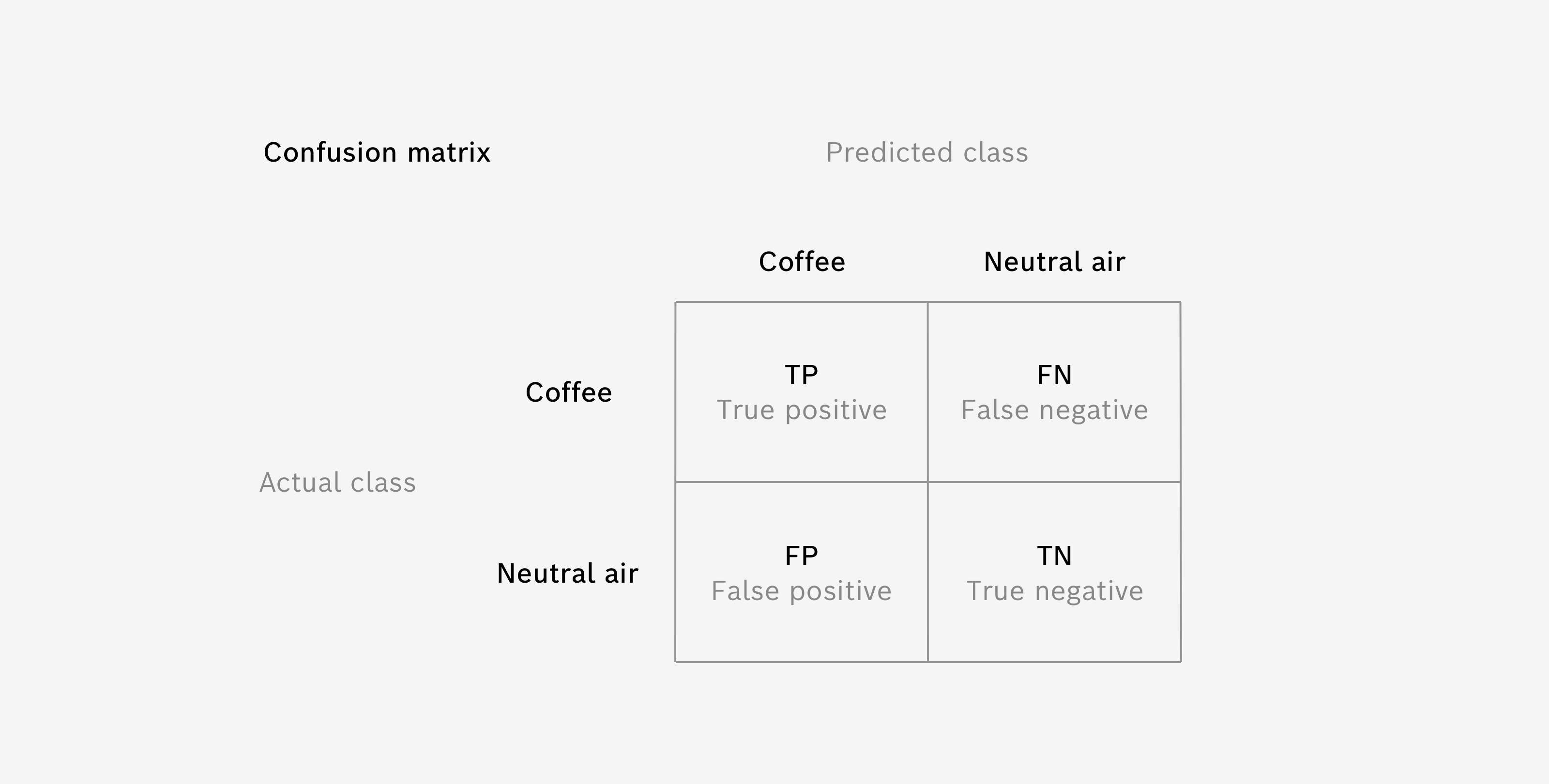
The Confusion Matrix also helps you evaluate how severe errors are for your specific use case. False alarms in one or the other direction may be very different in their impact on your use case. For example, if you want to detect coffee to warn the user, who maybe has an allergy against coffee, the case where the algorithm missed to detect coffee (so called “False Negative case”) is much more severe than the opposite way, where you have an alarm, although there is no coffee involved (so called “False/Positive case”).
Prediction Histogram
The Prediction Histogram is used as a detailed performance analysis for Regression algorithms.
It uses the Validation Data, which was set aside prior to training and not used during the training process (see Data Splitting). The histogram displays the distribution of prediction errors, meaning the differences between the predicted and actual values.
In an ideal scenario, where all predictions are precisely accurate, the histogram would show a single bar at zero, indicating no errors. However, in real-world scenarios, the errors typically follow a distribution around zero.
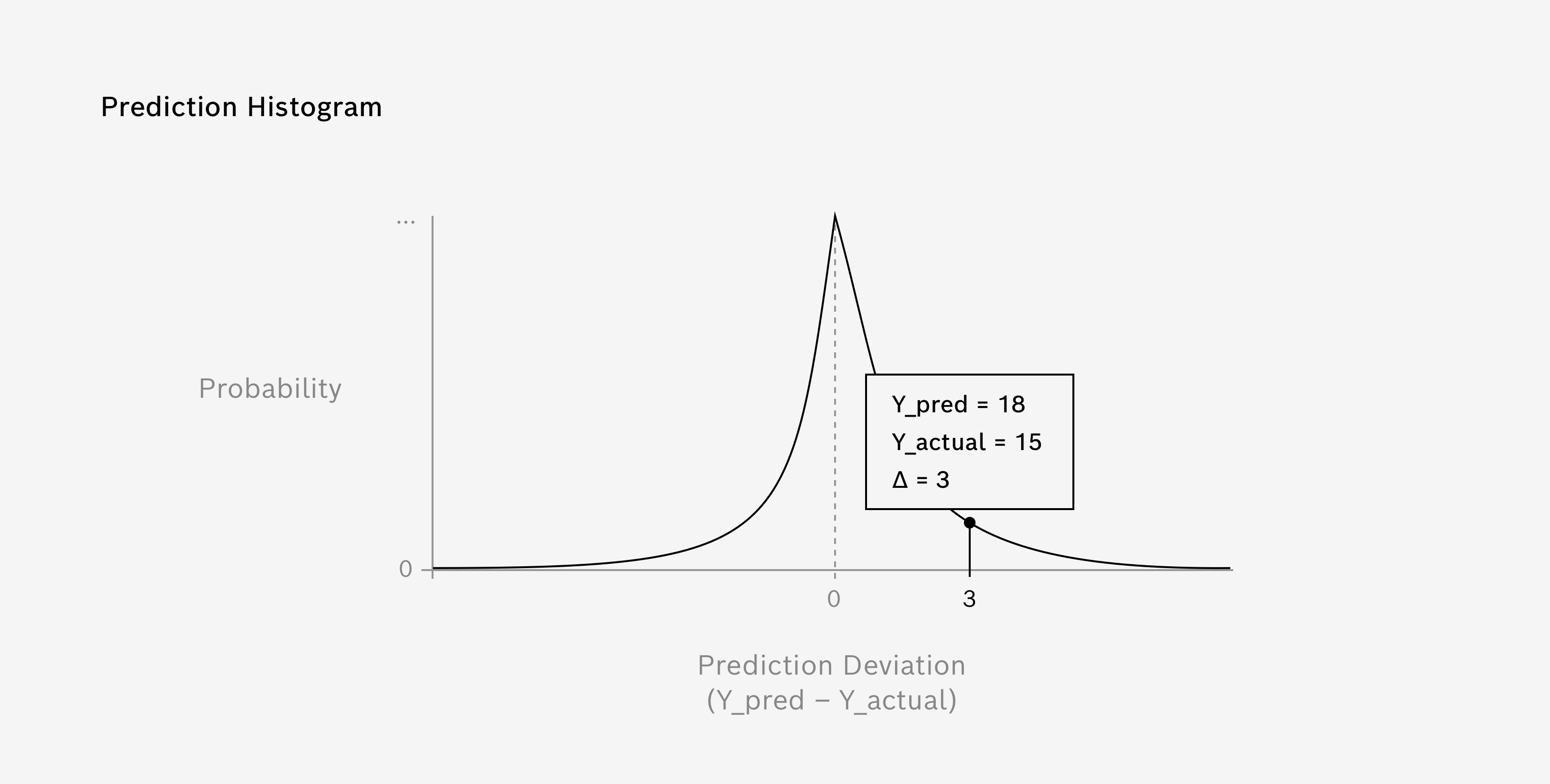
The Prediction Histogram can also assist you in understanding the impact of prediction errors for your specific use case. For instance, in a temperature forecasting model, underestimating the temperature (a negative prediction error) might have different consequences than overestimating it (a positive prediction error). This understanding will help you make necessary adjustments to your model or prepare appropriate mitigation strategies for the errors.
Additional Testing
After training your Algorithm, you can perform further tests of your Algorithm using additional data from your Specimen Collection. These tests are meant to be conducted with Specimen Data, which have not been used during the training of the Algorithm, in order to give insight on how the Algorithm performs with previously unknown or completely different data, that you do not want to include in the training process. This helps you estimate the robustness of the Algorithm, when facing exotic and unknown data.
To perform an additional test, simply select Test Algorithm. A new overlay opens that allows you to associate new, additional Specimen Data – the data you want to test. Once you have associated Specimen Data for Testing, you can select Run Tests.
Please note
As of this version of BME AI-Studio, additional tests and their results are not stored within your project. You can, however, save the results as a CSV-File by selecting Save Results.
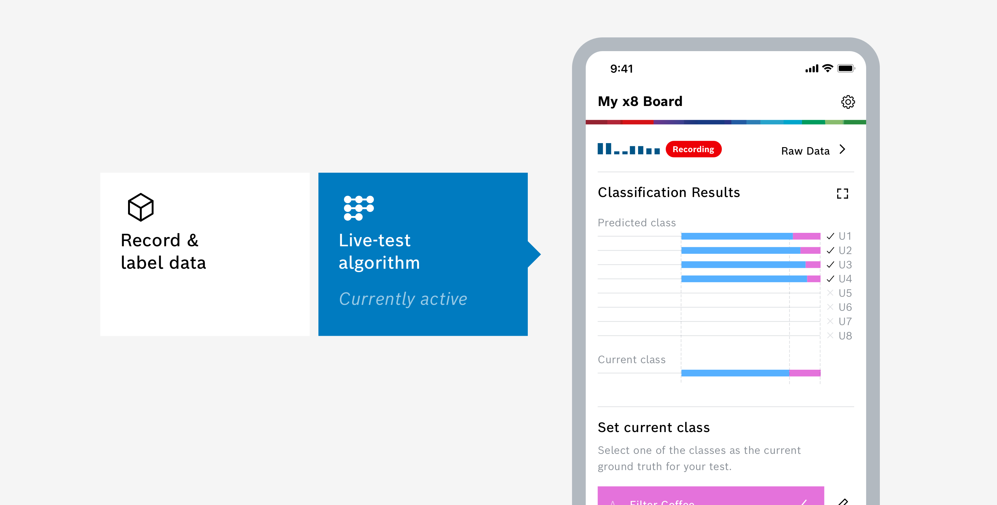
Live-Test with Mobile App
You can use the BME AI-Studio Mobile App to live-test your algorithm in the field. Install the app and connect to your BME688 Development Kit. Once connected, you can choose between two modes of operation – select Live-test Algorithm.
For more information about using the app during recording, please take a look here: Mobile App.
Algorithm Improvements
Too little variance
Having too little variance in the training data implies that the data lacks diversity and comprehensive representation of the scenario the algorithm is expected to handle. As a result, the trained algorithm may perform well on similar data but struggle with data points that are distinct or outside the range it was trained on - this phenomenon is known as overfitting. Essentially, the algorithm becomes too specialized in the narrow context of the training data and fails to generalize well to new, unseen data, which can lead to poor predictive performance and reliability when deployed in real-world applications.
An example: You want to distinguish coffee from normal air and you trained your classification algorithm with data from freshly opened coffee only. So that means, the neural net only knows the smell of fresh coffee compared to normal air and you are probably getting great results with high accuracies and F1 Scores, as well as low False/Positive rates. However, this does not necessarily imply that the algorithm would give you a great performance in all coffee situations. It only means that in this special situation (with freshly opened coffee) you are achieving good performance. So in order to get meaningful performance evaluations as well as effective training, it is important to reflect the variance of different situations also within the data recording used for training.
Too much variance
On the other hand, having too much variation in the training data implies a wide range of diversity and complexity within the dataset. This could make it challenging for the algorithm to discern underlying patterns and relationships, potentially leading to underfitting. Underfitting occurs when the model is too simplistic to capture the complexity in the data and consequently performs poorly on both the training and unseen data. The model's predictions may be inaccurate as it fails to sufficiently capture and learn from the diverse patterns and relationships present in the data, leading to suboptimal performance in real-world scenarios.
An example: If your neural net performance is very low, you might try to reduce the variance of the data and experiment with different subsets of the original data used for training. This might lead to better performance results, which give you some indication on which situations are very easy to handle for the algorithm and which are not.