V. Train Algorithms
Overview
Within the section My Algorithms you are able to use the data collected in your Specimen Collection to train algorithms. You are able to create multiple algorithms with a different data basis and individual settings. Once trained you can compare the performance of the different algorithms and choose the one algorithm that fits best to your use case (see Evaluate Algorithms).
An algorithm can be exported as a configuration file for the BSEC Software, which is basically a set of specific settings for the sensor and microcontroller, that enables the system to run the algorithm.
Create new Algorithm
First switch to My Algorithms, then select New Algorithm to create a new Algorithm. On the left you will see all your algorithms in a list view.
See Algorithm details
Once you select an algorithm within that list of algorithms, detail information of the selected algorithm is shown on the right hand side. Make sure you select Algorithm Settings. Here you can set up everything for the training of your Algorithm.
Train Algorithm
After setting up your algorithm, you can click Train Algorithm to start the training. Depending on the amount of data, the training can take from a few seconds up to several minutes. After the training, you can see the training results under Training Results. Jump to Evaluate Algorithms for further information.
Duplicate Algorithm
Once you select an algorithm, you can duplicate that algorithm, if you want to repeat your training with slightly different settings. Just click Duplicate Algorithm on the bottom of the screen or via the context menu by clicking ....
Delete Algorithm
Once you select an algorithm, you can delete that algorithm by clicking Delete Algorithm on the bottom of the screen or via the context menu by clicking ....
Algorithm
Name
Give your algorithm a name. Choose a name that might help you to identify and distinguish your Algorithms later on.
Created
The date and time you created that algorithm.
Type
BME AI-Studio supports two fundamental types of supervised learning algorithms: Classification and Regression algorithms.
Classification algorithms are used when the predicted quantity is categorical and discrete in nature. In other words, it is used when the data can be classified into different categories (called classes). For example, a classification algorithm can be used to distinguish "Espresso" from "Filter Coffee" based on the gas data.
Regression algorithms are used when the predicted quantity is continuous and numerical. In other words, it is used when the data can be measured as a number (called regression target). For example, these algorithms are used to predict quantities such as the concentration of a specific gas or let's say the amount of caffeine within different types of coffee. The numeric quantity is provided by the Meta Data keys.
The main difference between classification and regression lies in the type of output they provide. Classification predicts the category to which a new data point belongs, while regression predicts a continuous value. Choosing between classification and regression depends on the nature of your target variable. If your target variable is categorical, you use classification algorithms. If your target variable is numerical and continuous, you use regression algorithms.
Classification Data
Classes
Classes are the most important part of your Classification algorithm. Each class represents one of the different gas compositions you want to distinguish in your use case. For example, if you want to distinguish apples and oranges, you would create two classes – one class for apples, one class for oranges.
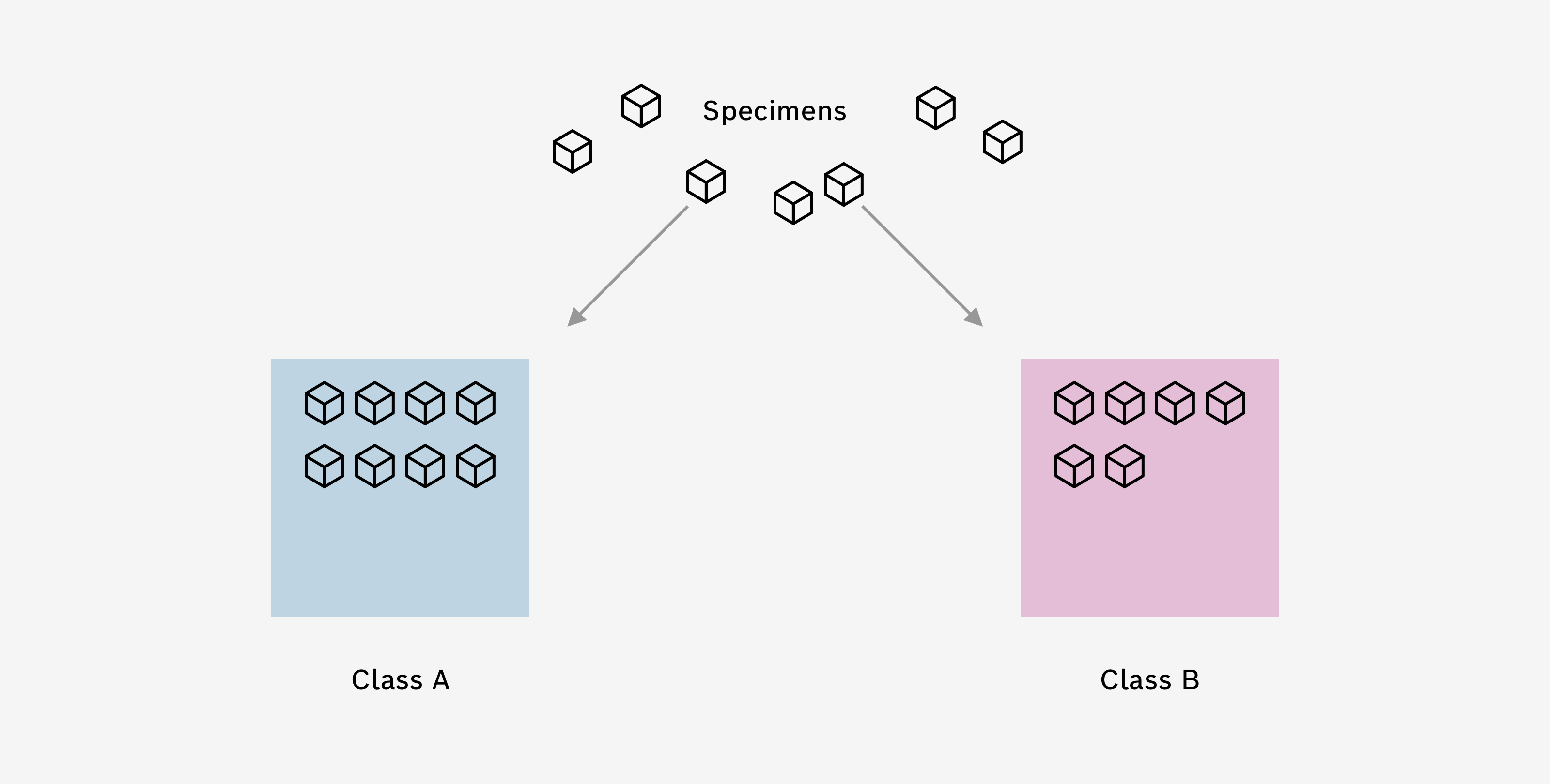
Once you created a class, you can then select Specimens from your Specimen Collection to add to that class. For example, if you recorded data from five different apples, you would add these Specimens to your apple class. And Specimens where oranges have been recorded, would be added to your oranges class.
Give your class a name that describes the gas composition you want to distinguish. Additionally, you can give your class a color of your choice.
Common Data
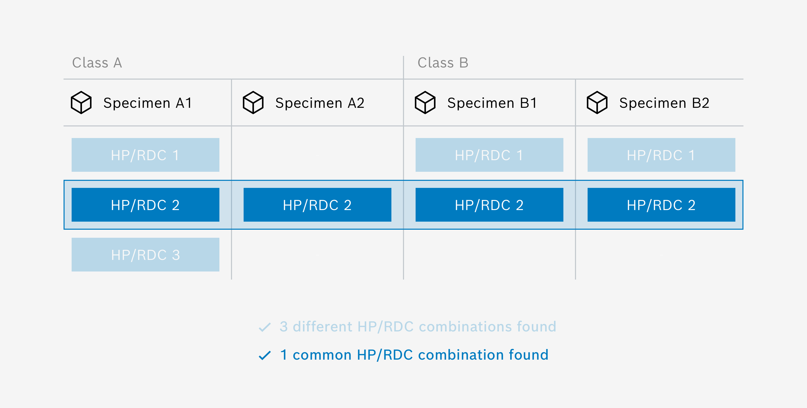
After adding specimens to your classes, BME AI-Studio checks the underlying data for common combinations of Heater Profiles and Duty Cycles (HP/RDC Combinations). This section shows if and which HP/RDC combinations were found in all specimens. If common HP/RDC combinations are found, a small check mark is displayed, which means that everything is OK.
Good to know: Selection rules for common HP/RDC
Each specimen can have data for one or more HP/RDCs. Algorithms can only be trained for HP/RDCs that are present in all specimens (that have been assigned to the algorithm classes). This means that the number of algorithms to be trained is calculated from the number of common HP/RDCs found in all specimens.
Data Balance
The graph shows how the summed durations of the gas data from the selected specimens are distributed across the classes. Ideally the distribution should be balanced. If there is a little checkmark, everything is okay and the data is balanced enough for training.
How Data Balance is calculated
Each class consists of multiple Specimens and each Specimen has a duration. The application checks if the total duration (sum of all Specimen durations) of any of the classes is below the following threshold:
threshold = 24% / number of classes
E.g.
- threshold for 2 classes: 12%
- threshold for 3 classes: 8%
- threshold for 4 classes: 6%
Regression Data
Regression Targets
Targets are the most important part of your Regression algorithm. Each target represents one numeric quantity you want to predict in your use case. For example, if you want to predict the caffeine content of different coffees, you would create a regression target that is connected to the caffeine Meta Data key.
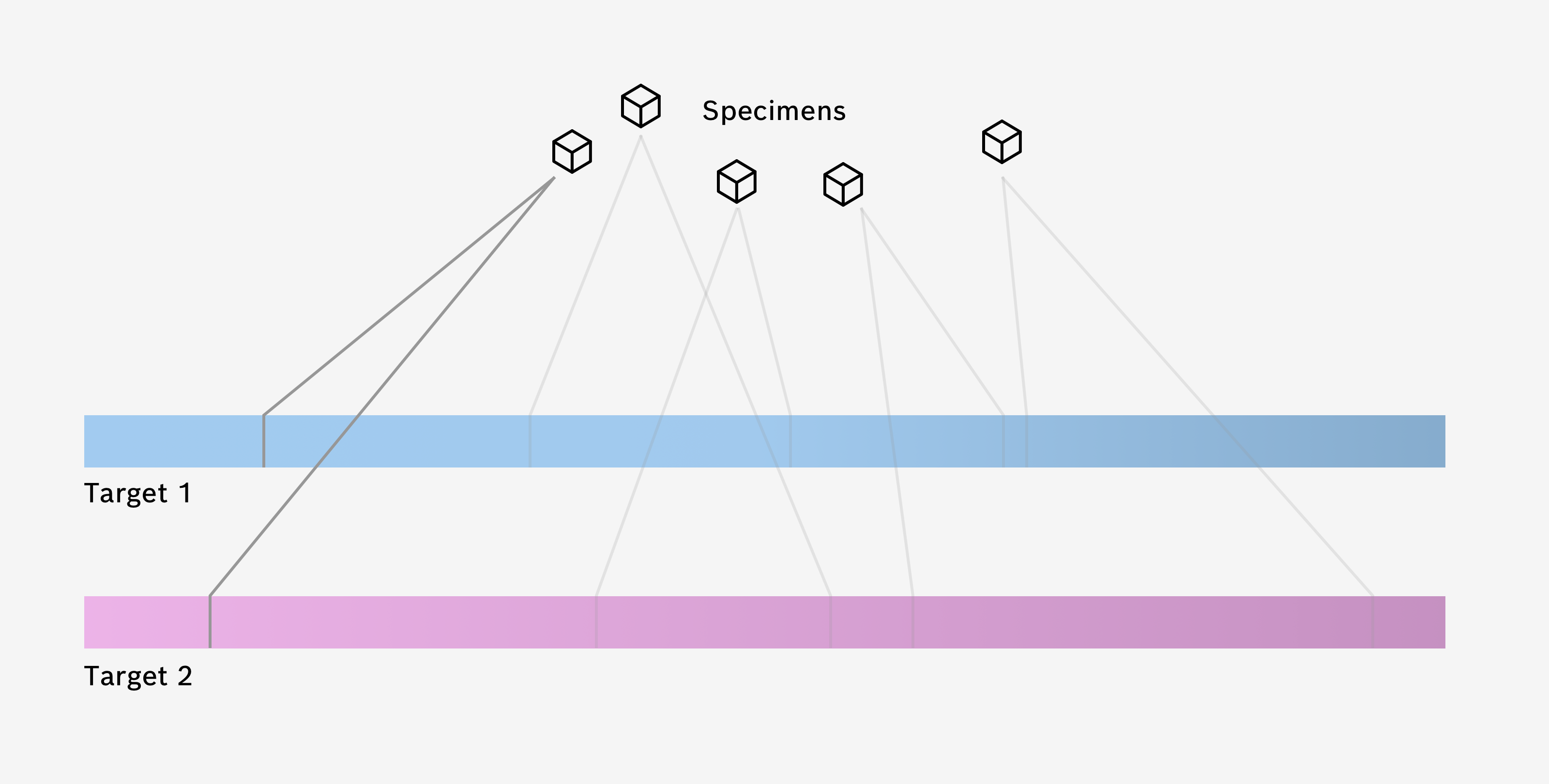
Once you created a regression target, you can then select a Meta Data key from a list of all Meta Data Keys in the project to be associated with that target. Additionally, you can give your target a color of your choice.
Specimen Data
By clicking on + Add Specimen a new overlay opens that lets you select Specimens from your Specimen Collection to be added to the regression algorithm.
Please note
You can only add Specimens to the regression algorithm that have numeric values for all Meta Data keys, which are selected as regression targets.
Common Data
After adding specimens to your Regression algorithm, BME AI-Studio checks the underlying data for common combinations of Heater Profiles and Duty Cycles (HP/RDC Combinations). This section shows if and which HP/RDC combinations were found in all specimens. If common HP/RDC combinations are found, a small check mark is displayed, which means that everything is OK.
Data Balance
The graph shows how the summed durations of the gas data from the selected specimens are distributed across the Regression target. Ideally the distribution should be balanced (all bins should have a similar duration). If there is a little checkmark, everything is okay and the data is balanced enough for training.
Please note
If you have selected too little data (in the form of specimens) the data balance can not be calculated.
How Data Balance is calculated
Each Specimen has Meta Data for each Regression target (Meta Data key). The different values are binned in up to 10 bins. The application checks if the normalized entropy (which can be understood as an expectation value for log(p), weighted with p and then summed over all bins) is above the following threshold:
normalized entropy: nH > 70%
Formally this is done by the following steps:
- Normalize the histogram Divide all bin durations by the total duration to get a probability distribution. The sum of all probabilities is equal to 1.
- Calculate entropy The entropy H of a probability distribution P = {p1, p2, ..., pn} can be calculated using the following formula:
H(P) = - Σ (p_i * log2(p_i))
for all i from 1 to n. In this formula, p_i is the probability of each bin (obtained in step 1), log2 is the base-2 logarithm, and Σ is the sum over all bins. - Normalize the entropy by dividing by the entropy H the maximum Entropy Hmax
nH(P) = H(P) / H_max(P) = H(P) / log2(n)
The normalized entropy will be 100% when all bins have the same duration (i.e., the histogram is uniform), which signifies a perfectly balanced histogram. Imbalance will lead to lower entropy values.
Data Settings
Data Channels
Specimen Data includes four data channels. You can choose, which Data Channel of each Specimen should be part of the training:
Gas Data Channel (10 data points)Humidity Data Channel (1 data point)Temperature Data Channel (1 data point)Barometric Pressure Data Channel (1 data point)
By default, only the Gas Data Channel is used for training. If other channels play a key role in your use case, you can try to include additional channels in the training and compare the training results.
Please note
Be careful with using additional channels for your training. Using additional Data Channels does not automatically mean better training results. The algorithm might focus only on one of the additional Data Channels during training, which might not be what you actually want. E.g. if one of your recorded Specimens has a strong impact on humidity, the algorithm might only focus on the correlation between the Specimen and the corresponding rise in humidity, ignoring all other data. Your training results may look very good, but the algorithm only “learned” to distinguish your Specimen by looking at the humidity, completely ignoring the respective gas data.
Please note
Be aware that including the Temperature Data Channel and Humidity Data Channel needs careful attention, since the temperature and relative humidity may not directly reflect the environmental conditions. This is due to the fact that both values are measured inside the metal packaging, which can be affected by self-heating effects of the BME688. For example running the sensor in a continuous cycling leads to a significant temperature increase inside the metal packaging and thus to a decrease of the relative humidity. This introduces transient effects on the recorded data, that do not originate from the actual sample you are measuring and therefore may mislead the training of the algorithm.
Please note
Be aware that including the Barometric Pressure Data Channel may introduce unwanted side effects. Since the barometric pressure signal is changing with your local weather, this may have an uncontrolled influence on the training process. Only include the Barometric Pressure Data Channel if you are sure that different Specimens or situations differ in their barometric pressure signal.
Data Filtering
The Apply clipping prevention option allows you to filter the data used to train the algorithm. If this option is enabled, all data points recorded with a heater profile step temperature below 125 °C (which could cause data clipping) will be ignored for training.
In general, enabling this option makes the algorithm more robust, especially to stabilization effects of the BME688 as well as special environmental conditions such as those encountered outdoors.
Why to avoid data from heater steps with low temperatures?
When the BME688 is operated at relatively low temperatures (e.g. < 125 °C), the raw gas resistances are quite high and close to the clipping threshold of the internal analog-to-digital converter. Under certain circumstances, this can lead to clipping of the data. Even if the data is not clipped within the training data, stabilization of the sensor can lead to higher raw gas resistances, so clipping may occur in the future.
Because these clipping effects can confuse trained algorithms - especially if the algorithm is trained with relatively new sensors (without clipping) and later run with aged sensors (with clipping) - this can lead to algorithm performance problems.
This does not mean that clipping data points (caused by low temperature Heater Profile steps) are useless. In fact Heater Profiles with low temperature steps can trigger certain chemical effects that can then be investigated at subsequent higher temperature steps.
Data Augmentation
The Generate aged sensor data option allows you to generate additional training data that will ultimately make your algorithm more robust to sensor aging effects. In addition, this feature can also be useful to improve generalizations related to sensor-to-sensor variance.
This feature uses a specially designed mechanism to artificially age existing sensor data and use this data (in addition to the data you recorded) for training the algorithm. You can set up to which Maximum age data should be generated. You can choose from 18 months, 60 months and 120 months. The data augmentation happens in 6 so called Augmentation steps (interim steps). For every augmentation step additional data will be generated for the respective age. For example, if a Maximum age of 18 months is selected data will be generated for 3, 6, 9, 12, 15 and 18 months. Effectively this leads to a multiplication of the data by factor 7.
The table below shows the augmentation steps for each Maximum age:
| Maximum Age | Augmentation steps |
|---|---|
| 18 months | 3, 6, 9, 12, 15 and 18 months |
| 60 months | 10, 20, 30, 40, 50 and 60 months |
| 120 months | 20, 40, 60, 80, 100 and 120 months |
On the reproducibility of training with data augmentation
The (artificially generated) augmented data is not stored long-term in the project. Since the mechanism used to generate the data is deterministic, the initial training condition (with respect to the augmented data) can be reproduced by duplicating the algorithm.
However, since the data augmentation mechanisms developed by Bosch are under continuous development, newer versions of BME AI-Studio may include improved mechanisms. This does not ensure reproducibility of training output conditions with respect to data augmentation across different versions of BME AI-Studio.
Choose other Neural Nets
In the current version of BME AI-Studio you can choose one pre-defined Neural Net Architecture. In a future release we plan to have the possibility to chose other architectures.
Training Settings
Training Method
Choose the training method for the training. In this version of BME AI-Studio, only one optimizer function is available (ADAM optimizer). You can choose between different batch sizes:
- ADAM optimizer, batch size 4
- ADAM optimizer, batch size 16
- ADAM optimizer, batch size 32
- ADAM optimizer, batch size 64
Batch size in neural network training refers to the number of data samples the algorithm processes together in each step. Adjusting this size can affect how quickly and smoothly the training progresses.
Generally, using a larger batch size can speed up the training and make it more consistent. However, there's a trade-off. With a larger batch size, there's a higher risk of the algorithm getting 'stuck' at a suboptimal solution, known as a 'local minimum'. This means the algorithm finds a solution that seems best within a limited view but isn't the overall best or 'global' solution. On the other hand, a smaller batch size reduces this risk, potentially leading to better overall results, but the training might be slower and less stable.
Max. Training Rounds
A training round (or epoch) in machine learning is a complete pass through the entire training dataset where the model's weights are updated to improve its predictive accuracy.
The higher the number of (maximum) training rounds for the training, the longer the training can take. If you are not limited by the computation time choose a higher number of training rounds.
Data Splitting
Training data is the initial set of information used by BME AI-Studio to learn patterns, rules, or behaviors, providing a foundation for its prediction capabilities. Validation data, on the other hand, is a separate subset of data not used in training, which helps in evaluating the model's performance during training, ensuring that the model is learning correctly and not merely memorizing the training data.
Choose which fraction of the data should be used for training and validation respectively.
Please note
This is an expert setting. If you wan't to know more about Data Splitting, please get in touch with us.
Loss Function
For Classification algorithms there is a fixed loss function
- Cross Entropy Loss is a type of loss function commonly used in machine learning multi-class classification problems. In these problems, the outputs are categorical, meaning they take on a fixed set of values, each representing a different class:
Cross Entropy Loss = - Σ (y_actual * log(y_pred))
For Regression algorithms there are two options for loss functions
L1 Loss (also known as Least Absolute Deviations or LAD) is a type of loss function commonly used in machine learning regression problems. It is defined as the sum of the absolute differences between the actual value and the predicted value:
L1 Loss = Σ (|y_actual - y_pred|)
L1 loss is robust to outliers, meaning it doesn't drastically change the model's predictions when there are outliers in the data. But, it might lead to unstable solutions, as small changes in the data can lead to large changes in the model's parameters.L2 Loss (also known as Least Squares Error or LSE) is a type of loss function commonly used in machine learning regression problems. It is defined as the sum of the squared differences between the actual value and the predicted value:
L2 Loss = Σ ((y_actual - y_pred)^2)
Unlike L1, L2 loss is not as robust to outliers because squaring the differences amplifies the effect of large errors. On the positive side, L2 loss provides a more stable solution numerically (i.e., small changes in the data lead to small changes in the model's parameters). This leads to simpler and possibly more interpretable models. L2 is selected as the default loss function for Regression Algorithms.
Training in progress
While the training of the algorithm is in progress, you are provided with detailed information on the following measures:
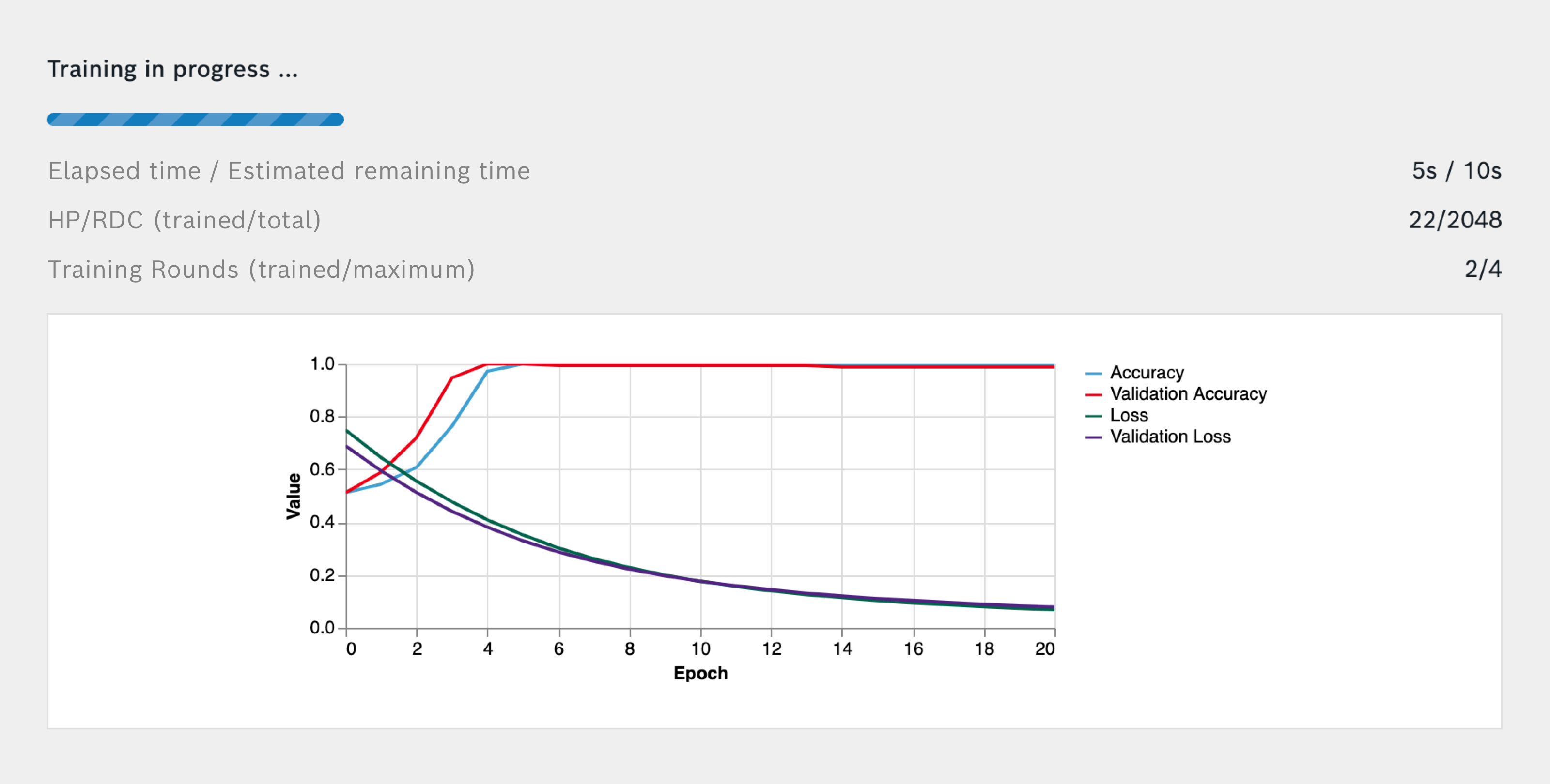
- Elapsed time since the beginning of the training
- Maximum remaining time that it takes to finish the training (Calculation is based on number of training rounds. This is a worst case estimation, training is typically much shorter.)
- Number of already trained HP/RDC Combinations
- Total number of HP/RDC Combination to be trained for this algorithm
- Number of already trained Training Rounds
- Maximum number of Training Rounds to be trained for this algorithm